-
Nozzle Local Stress Assessment
In most cases, nozzles installed on a pressure vessel obtained external loads composed with forces and moments throughout the plant operation. This particular condition might impair the structural integrity of the nozzle once it is not carefully devised and maintained. Thus, further analytical assessment based on standardizations and codes is invariably conducted. Initially, while designing pressure vessels and nozzles in a construction stage, ASME Section VIII is used to provide details of the design which can withstand against the operational loads like the internal pressure, as such the nozzles are considered safe to be operated. However, the ASME section VIII merely addresses specific cases and does not cover all desired cases which require to evaluate the integrity of the nozzles throughout the operation, for instance, external loads consideration is not fully addressed in this code, thereby, one needs to delve beyond this code to design safe attachments on the vessels due to external loads.

Figure 1. Loads acted on a nozzle
Since Welding Research Council (WRC) 107 bulletin was published in 1965, this code is used as the additional nozzle assessment to determine stresses emerged on the spherical and cylindrical shells due to nozzle attachments. Furthermore, WRC 297 was issued to provide better engineering evaluation, whereby, this bulletin furnishes stress calculation and stress intensity on both nozzle and shell sides. Both WRC bulletins published neglect the effect of the internal pressure [1] and predominantly concentrate on the integrity assessment due to the applied external loads.
Despite the simplified method offered by WRC procedures to evaluate the stress on both the nozzle and vessel, there are some issues arise. First, WRC 297 is prone to generate poor overstress results at the nozzle side instead of at the shell side [1]. Secondly, geometric limitations become another issue which obstructs W RC 297 to be used extensively, as such application for a large diameter nozzle might lead to non-conservative results [3]. Thirdly, when designing a vessel head with multiple adjacent nozzles, then the WRC is not fully capable to simultaneously calculate the accurate stress results. Therefore, in order to overcome blind spots of WRC, Finite Element Analysis is often opted to be used as the comparison [2] to justify the previous analytical calculation using WRC as depicted in Figure 2.

Figure 2. Stress Intensity Comparison between WRC and FEA [3]
REFERENCE
[1] Chandiramani, D., Nawandar, S.K., Gopalaskrishnan, S. 2013. Stresses In Nozzle Shell Junctions Due To External Loads – A Comparative Study. Proceedings of the ASME 2013 Pressure Vessels and Piping Conference
[2] Lee, H.S., Ha, C.H., Park T.J. 2011. Finite Element Analysis For Nozzle With External Loads. Proceedings of the ASME 2011 Pressure Vessels & Piping Division Conference.
[3] Chema, R.M., Patel A.N., Alam A. 2019. Analysis of Pad Reinforced Openings in Pressure Vessels. International Journal of Engineering Research & Technology (IJERT).
-
Evaluation of Dissimilar Weld Joints
Dissimilar Weld Joint (DWJ) is commonly found in oil and natural gas industry, power plant, and nuclear industry. This integration between two different materials aims to reduce equipment weight and increase the properties of materials, notably its corrosive behaviour. The differences of properties between these materials generate different responses under several conditions. Properties such as the linear expansion coefficient and thermal conductivity might affect the emergence of stress which initiates the formation of crack on metal surfaces [6]. Thus, understanding this behaviour is essential to evaluate and estimate its remaining useful life to prevent failure during the operation.
In offshore industry, DWJ is encountered on fittings of pipeline. As can be seen in figure 1, this process of integrating a different material of Inconel 625 is called buttering. This Ni-based alloys are corrosion resistance alloys that are extensively utilized in adverse H2S environments that also contain high temperature and high pressure[3]. Buttering is imperative in welding connection since welding directly carbon steel materials to stainless steel materials poses reduction of corrosion resistance in low carbon materials (stainless steel). Therefore, buttering aims to minimize the risk of this occurrence. Figure 2 depicts a study from Daniel et al [1] which scrutinized 3 different materials, including A-36, 8630M and Inconel 625 with the Finite Element Method (FEM). The results of analysis could predict the behaviour of stress and strain fields related to cracks in the sample.

Figure 1. Dissimilar Weld Joints in Fittings [5]
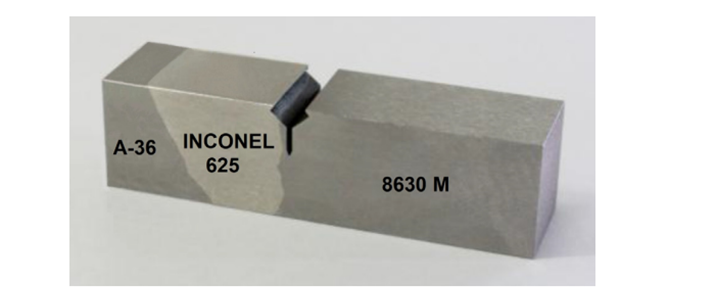
Figure 2. Experimental study to investigate crack propagation in Dissimilar Weld Joints [1]
Due to the different properties given by each material, DWJ could generate uneven distribution stress leading to initiation of crack. The localized stress posed by this uneven distribution can be an initial point where crack occurs, thus, this situation reduces its fatigue life especially when it is subjected with cyclic loadings. In order to diminish the likelihood of failure due to crack propagation, one of the methods used is to reduce the residual stress emerges in this joint [4]. For example, a study from Alhafadhi et al [2] investigated the influence of heat input to the residual stress, whereby, low heat input contributed to lower residual stress as can be seen in Figure 3.

Figure 3. Effects of heat input to residual stress [2]
REFERENCES
[1] Daniel N.L. Alves, José G. Almeida, Marcelo C. Rodrigues.2020. Experimental and numerical investigation of crack growth behavior in a dissimilar welded joint.Theoretical and Applied Fracture Mechanics, Volume 109, 102697, ISSN 0167-8442,
[2] Alhafadhi, M., Krallics, G. 2020. Finite Element Modelling Of Residual Stresses In Welded Pipe Welds With Dissimilar Materials. Materials Science and Engineering, Volume 45, No. 1 (2020), pp. 7–19
[3] Chengshuang Z., Qiuyan H., Qiang G., Jinyang Z., Xingyang C.n, Jun Z., Lin Z.2016. Sulphide stress cracking behaviour of the dissimilar metal welded joint of X60 pipeline steel and Inconel 625 alloy. Corrosion Science,Volume 110,Pages 242-252,mISSN 0010-938X,
[4] Jiang, W., Luo W., Li, J.H., Woo, W.2017. Residual Stress Distribution in a Dissimilar Weld Joint by Experimental and Simulation Study. Journal of Pressure Vessel Technology
[5]Ibrahim, S.E.2020. Effect Of High Pressure High Temperature And Sour Service Environment On Subsea Dissimilar Joints. Inspectioneering Journal
[6]Wang, B., Lei, B,B., Wang,W., Xu,M., Wang,L. 2015. Investigations on the crack formation and propagation in the dissimilar pipe welds involving L360QS and N08825. Engineering Failure Analysis.
-
Advance Computational Models of Fracture Mechanics in Evaluating Structural Integrity of Equipment in Oil & Gas Industry.
Introduction
Structural Integrity of equipment in Oil and Gas Industry is a major issue which invariably encountered during all stages of operation. Pipeline, for instance, might be found defects due to fabrication or operating services which may deteriorate its remaining useful life. The importance of assessing the integrity of these equipment needs to consider underlying physic of fracture mechanics since one could determine pertinent parameters contributed to failure phenomena such as crack propagation. Failure of equipment due to crack propagation can be induced by several factors such as internal pressure, corrosion, or pre-existing dents. Furthermore, this phenomenon could emerge in surfaces of equipment or in weld joints, in particular circumferential weld joints which are considered as weakest links in pipeline [2]. In which, crack occurs when a critical parameter in fracture mechanics such as Stress Intensity Factor (SIF) or J-Integral reaches its critical value. For example, figure 1 exhibits interplay between SIF and Crack Growth Rates (m/s), whereby high SIF proportionally leads to higher crack growth rates

Figure 1. SIF and Crack Growth Rate [3]
Roles of Advance Computational Models
Intricate loading conditions in oil and gas industry prompts robust analysis methods to provide more accurate results. Conventional Finite Element Method (FEM) presumably has shortcomings in generating desirable results in cumbersome cases like crack propagation due to its computational cost and outcomes of analysis could be mesh-dependent leading to discrepancies towards the results when size of mesh is modified [5]. Additionally, crack propagation considers a wide range of parameters to fully represent its physic phenomenon. Therefore, several advance computational models in predicting crack propagation are proposed, including Extended Finite Element Method (XFEM), Gurson Tvergaard-Needleman (GTN), Fracture Locus Curve (FLC), Cohesive Zone Model(CZM) etc. Nonn et al, attempted to compare 3 models in analyzing ductile crack propagation with GTN, FLC, and CZM as can be seen in Figure 2, where proper results could be produced once parameters of models were set appropriately [7]

Figure 2. Crack Simulation between 3 Different Models [7]
Cohesive Zone Model (CZM)
Among other models, CZM is arguably a common model used to evaluate crack propagation in fracture mechanics. In CZM, damage of materials is initiated when the cohesive traction is zero [5]. Herein, cohesive forces in a cohesive zone would play critical roles in resisting crack to grow larger. A main objective of harnessing this model is to encounter a parameter namely Crack-Tip Opening Angles (CTOA) where this parameter has acquired broad acceptance to be used as a fracture-resistance parameter by ASTM and ISO [4]. Indication of crack propagation can be obtained when there is a change of CTOA. CTOA signifies a driving force required to make crack propagation, where CTOA also indicates the toughness of materials. Figure 3 shows a relationship between CTOA and crack length, where a material TH4 possessed larger fracture energy by 15.188 (MPA.mm) compared to a material TH3 (14.580 MPa.mm) ,TH2 (14.175 MPa.mm) ,and TH1 (12.150 MPa.mm), as can be concluded higher CTOA could be found in the material with bigger fracture energy [4]

Figure 3. CTOA and Crack Length [4]
References
[1]Xiaohua Zhu, Zilong Deng, Weiji Liu, Dynamic fracture analysis of buried steel gas pipeline using cohesive model, Soil Dynamics and Earthquake Engineering, Volume 128, 2020,105881,ISSN 0267-7261,https://doi.org/10.1016/j.soildyn.2019.105881.
[2] Polasik, S. J., Jaske, C. E., & Bubenik, T. A. (2016). Review of Engineering Fracture Mechanics Model for Pipeline Applications. Volume 1: Pipelines and Facilities Integrity. doi:10.1115/ipc2016-64605
[3] Matvienko, Y. G. (2011). A Damage Evolution Approach in Fracture Mechanics of Pipelines. NATO Science for Peace and Security Series C: Environmental Security, 227–244. doi:10.1007/978-94-007-0588-3_15
[4] Dunbar, A., Wang, X., Tyson, W. R., & Xu, S. (2014). Simulation of ductile crack propagation and determination of CTOAs in pipeline steels using cohesive zone modelling. Fatigue & Fracture of Engineering Materials & Structures, 37(6), 592–602. doi:10.1111/ffe.12143
[5] Shahzamanian, M. M., lin, M., Kainat, M., Yoosef-Ghodsi, N., & Adeeb, S. (2021). Systematic literature review of the application of extended finite element method in failure prediction of pipelines. Journal of Pipeline Science and Engineering, 1(2), 241–251. doi:10.1016/j.jpse.2021.02.003
[6]Nie, H., Ma, W., Sha, S., Ren, J., Wang, K., Cao, J., & Dang, W. (2020). Dynamic Impact Damage of Oil and Gas Pipelines. Journal of Physics: Conference Series, 1637, 012094. doi:10.1088/1742-6596/1637/1/012094
[7] Nonn, A., & Kalwa, C. (2012). Simulation of Ductile Crack Propagation in High-Strength Pipeline Steel Using Damage Models. Volume 3: Materials and Joining. doi:10.1115/ipc2012-90653
-
Machine Learning Models for Predicting Carbon Emissions
Carbon emissions are arguably predominant causes of global warming which poses the increase of temperature on earth. Whereby, IPCC predicts subsequent inclination of temperature until 1.5oC between 2030 and 2052 based on the current rate [1]. Recently, all countries attempt to reduce the carbon emissions by proposing several approaches, in particular China which possesses the larger share of carbon emissions compared to other countries as can be seen in figure 1 [6]. Thus, measurement of carbon emissions is an imperative step to assess the effectiveness of efforts made by all parties including government and stakeholders. In order to appraise the carbon emissions, CO2-equivalents (CO2eq) is a common variable used to evaluate the impact of CO2 to global warming [2]. However, carbon emissions are influenced by a multitude of factors, hence these complex systems pose difficulties in predicting the underlying impulse of the emissions. Lacks of understanding to major underlying causes of carbon emissions might lead to ineffective regulation or preventive actions, thus it’s utterly important to have a viable method to forecast the emissions [3].

Figure 1. Countries’ share of carbon emissions [6]
Recently, machine learning is extensively utilized to predict carbon emissions based on several factors. Sajid [4], scrutinized carbon emissions with other independent variables, including Gross Domestic Product (GDP), urban agglomerations, urbanization, fossil fuel consumption, and energy consumption, where the linear regression model outperformed ANN in this study and energy consumption had the highest affect with regression coefficients by 0.33345. Meng et al [5] proposed 4 different machine learning models to forecast carbon emissions rates in the future and study the effects of COVID19 on carbon emission rates, despite this study merely scrutinized a relationship between carbon emissions and years, however the author stressed the propose models had strong similarity with the IPCC model in predicting the emissions.
Study Case: a simple example of carbon emissions prediction
In order to delve the implementation of machine learning in predicting carbon emissions, in this article an understandable dataset from Kaggle is provided to train a machine learning model [7]. Herein, Gradient Boosting Regressor (GBR) was selected as the model to forecast the dependent variable which uses the ensemble method where we can incorporate various models to get better performance of the machine learning model.
The dataset consists of 74 features and a dependent variable of carbon emissions derived from 497 locations. Before training the model, correlation matrix was conducted as a statistical method to appraise the interplay between variables in our dataset which can be seen in Figure 2. Among 74 features, 72 features had no strong correlation with the dependent variable (carbon emissions).
The results showed that GBR predicted the output with R2 score by 0.77. Whereby in this case, this model was not well-performed to learn from the existing datasets. Further study needs to be conducted to train other machine learning models [7] such as Deep Neural Network, Artificial Neural Network, Support Vector Machine, Decision Tree Regeressor , etc to obtain better results. Moreover, in order to optimize the performance, hyperparameter tuning as a prolonged process can be done to get the optimal parameters that can help boosting the model performance.

Figure 2. Correlation Matrix of Variables in the Dataset.
REFERENCES
[1] IPCC, 2018: Summary for Policymakers. In: Global Warming of 1.5°C. An IPCC Special Report on the impacts of global warming of 1.5°C above pre-industrial levels and related global greenhouse gas emission pathways, in the context of strengthening the global response to the threat of climate change, sustainable development, and efforts to eradicate poverty [Masson-Delmotte, V., P. Zhai, H.-O. Pörtner, D. Roberts, J. Skea, P.R. Shukla, A. Pirani, W. Moufouma-Okia, C. Péan, R. Pidcock, S. Connors, J.B.R. Matthews, Y. Chen, X. Zhou, M.I. Gomis, E. Lonnoy, T. Maycock, M. Tignor, and T. Waterfield (eds.)]. Cambridge University Press, Cambridge, UK and New York, NY, USA, pp. 3-24, doi:10.1017/9781009157940.001.
[2] Simon Eggleston, Leandro Buendia, Kyoko Miwa, Todd Ngara, and Kiyoto Tanabe. 2006 IPCC guidelines for national greenhouse gas inventories, volume 5. Institute for Global Environmental Strategies Hayama, Japan, 2006.
[3] D. Cogoljevi´c, M. Alizamir, I. Piljan, T. Piljan, K. Prlji´c, S. Zimonji´c, A machine learning approach for predicting the relationship between energy resources and economic development, Physica A (2017), https://doi.org/10.1016/j.physa.2017.12.082
[4] M J Sajid 2020 IOP Conf. Ser.: Earth Environ. Sci. 495 012044
[5] Meng, Y.; Noman, H. Predicting CO2 Emission Footprint Using AI through Machine Learning. Atmosphere 2022, 13, 1871. https://doi.org/10.3390/atmos13111871
[6] Jena, P.M.; Managi, S.;Majhi, B. Forecasting the CO2 Emissions at the Global Level: A Multi‐layer Artificial Neural Network Modelling. Energies 2021 14, 6336. https://doi.org/10.3390/ en14196336
[7] Darius Moruri, Amy Bray, Walter Reade, Ashley Chow. (2023). Predict CO2 Emissions in Rwanda. Kaggle. https://kaggle.com/competitions/playground-series-s3e20
-
Reaction Forces Consideration in the Piping System.
Ensuring safety of a system in a plant is essential to impede any accidents throughout the operation, in particular several plants require strict demands for safety operation such as oil refinery and nuclear power plant. Maintaining equipment to be operated between its allowable limits is mandatory. Predominantly, stress analysis is conducted to attest the integrity of the equipment. In a plant, a reliable piping system is attained by designing the system that complies to common industrial standardizations such as ASME. One of the evaluation in this system is assessing the generated reaction forces on the pipe supports due to loads induced by the fluid inside the pipe because the magnitude of pressure inside the piping systems would increase the amount of reaction forces generated by the supports [1].

Figure 1. Safety Valves Installation [2]
The installation of fittings or valves in a piping system poses the reaction forces of the supports. The utilization of safety valves, for instance, must consider the design of the pipe length and the location of the valve as can be seen in Figure 1 because the blowdown process or when the safety valves relieve pressure from vessels would yield forces which could be distributed to the pipe rack structures near the safety valves and the reaction forces would get larger when the length of the blowdown pipe increases [2].
Due to the adverse effects generated by the reaction forces in the pipe supports, additional design of reinforcement isS proposed. For example, Jeong et al proposed a method in predicting the reaction forces in the Hydraulic Transfer System (HTS) of Kijang Research Reactor to design an embedded plate on pool lines as the reinforcement, hence this system could be safe once the occasional loads (earthquake) occur [3].
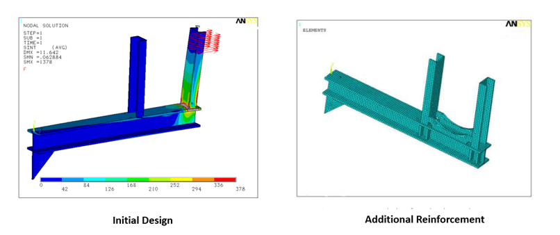
Figure 2. Pipe supports with additional reinforcement [4]
Dizdar et al [4] designed reinforcement plates for pipe structures of the nuclear piping systems as can be seen in Figure 2. The underlying reason of this design was the installed support could not satisfy the support design standardization based on ASME NF-3200, notably because the maximum force that the supports could withstand was 10.9 KN, however, the allowable limit was 7.3 KN. In lieu of replacing the existing support, additional plates were proposed to increase strength of the pipe supports.
Conclusion
The integrity of the piping supports due to the reaction forces induced by the loads of the piping system must be considered carefully, despite stresses generated by the pipes are acceptable. All previous studies substantiate the idea of predicting the reaction forces in the piping supports, thus, the future design of the supports will withstand against the operating loads in the system.
References
[1] Kitade et al.1979. Experimental Study of Pipe Reaction Force and Jet Impingement Load at the Pipe Break. Japan. International Conference on Structural Mechanics in Reactor Technology.
[2] Muschelkanuts,S. Wellenhofer,S. 2003. Flow Reaction Forces upon Blowdown of Safety Valves. Chemical Engineering & Technology.
[3] Jeong J., Oh, J. 2020. Prediction of Reaction Forces on the HTS Supports. Korea Nuclear Society Conference.
[4] Dizdar, S., Vucina, A., Rasovic, N., Tomovic R. 2018. Application of Pipe Stress and ANSYS in Stress Analysis of Nuclear Pipe Supports-Case Study. IOP Conf. Series: Materials Science and Engineering.
-
Is Finite Element-Neural Network a Quantum Leap in Assessing Corrosion Defects?

Introduction
Finite Element Analysis (FEA) was extensively utilized in engineering fields in mid 1950s, where this assessment method discretizes a complex geometry into small elements. This discretization method approximates Partial Differential Equations (PDEs) with numerical model equations. FEA entails several processes including modelling, meshing, processing, and post-processing. Recently, Artificial Neural Networks (ANNs) starts to be integrated with FEA in order to ease the processes of engineering analysis as can be seen in Figure 1. This integration can enable one to make immediate assessment by using past data thanks to the ability of ANN that works by emulating the neuron mechanisms in our brain which can learn, store, and classify information.

Figure 1. Integration between FEA and ANN.
FEA is used to generate datasets required to train ANNs for rapid computations, and this fusion surmounts a major impediment of FEA that needs a high amount of time to produce accurate results (high computational costs). Hence, in the future, the trained ANNs will be used to conduct rapid evaluation, thereby, engineers will not spend a lot of time to conduct recurrent analysis, notably when they will cope similar issues in the past. Additionally, this fusion enables the periodic assessment to be done because the integrity equipment is not supposed to be merely done when failures occur but it has to be done periodically, for example, in order to ensure safe operation of pipeline then the pipeline needs to be appraised from time to time [1-3].
Moreover, another issue solved by this incorporation is the ability to provide both rapid and accurate assessment. In a corrosion assessment method, for instance, some standardizations (ASME B31G, SHELL 92, PCORRC, etc) that govern this assessment are arguably conservative [4] leading to early reparation and unnecessary maintenance activities. Thus, robust assessment method is immensely required to overcome this issue.
FEA and ANN to Assess Corrosion Defects
Corrosion defects are predominantly encountered in carbon steel pipelines. This type of defects can occur in a single defect and interacting defects. Figure 2 depicts Interacting corrosion defects which can happen when there are two or more defects on pipelines, whereby these defects deteriorate strength of pipelines by diminishing failure pressures of pipelines [5]

Figure 2. Circumferential Defects on a Pipe [6].
An example of a study that scrutinized the fusion of FEA and ANN was conducted by Kumar et al [7], where they studied the integration between FEA and ANN to predict the failure pressures of X80 Pipeline. Artificial datasets from finite element simulation were produced to train ANN. The artificial datasets were created by varying geometric parameters of the defects such as defect spacing, defect length, defect, depth, and longitudinal compressive stress. Total 241 datasets were generated to train the ANN. Prior to producing these datasets the results of FEA were validated with burst tests in previous studies with errors by 2.46% for a case of interacting defects. The ANN model was assessed with R2 scores as metrics to evaluate the performance of model, as the result the trained model of ANN produced the highest R2 score by 0.999, which signified that the model could forecast the failure pressure on pipelines accurately.
Conclusions
As a conclusion, ANN is a sophisticated approach that can be incorporated with FEA to assess corrosion defects in equipment. In addition, this incorporation will arguably become a quantum leap in assessing defects in equipment because its latent potential to create rapid and accurate assessment.
References
[1] Dewanbabee, H.; Das, S. Structural Behavior of Corroded Steel Pipes Subject to Axial Compression and Internal Pressure: Experimental Study. J. Struct. Eng. 2013, 139, 57–65
[2] Li, X.; Chen, Y.; Zhou, J. Plastic Interaction Relations for Corroded Steel Pipes under Combined Loadings. In Proceedings of the 12th Biennial International Conference on Engineering, Construction, and Operations in Challenging, Honolulu, HI, USA, 14–17 March 2010; pp. 3328–3344.
[3] Seyfipour, I.; Bahaari, M.R. Analytical study of subsea pipeline behaviour subjected to axial load in free-span location. J. Mar. Eng.Technol. 2021, 20, 151–158
[4] Chiodo, M.S.G.; Ruggieri, C. Failure assessments of corroded pipelines with axial defects using stress-based criteria: Numerical studies and verification analyses. Int. J. Press. Vessel. Pip. 2009, 86, 164–176
[5] Adilson C. Benjamin, José Luiz F. Freire, Ronaldo D. Vieira, Divino J.S. Cunha, Interaction of corrosion defects in pipelines – Part 1: Fundamentals, International Journal of Pressure Vessels and Piping, Volume 144, 2016, Pages 56-62, ISSN 0308-0161,https://doi.org/10.1016/j.ijpvp.2016.05.007.
[6] Neesa, N.; Mustaffa, Z.; Seghier, M.E.A.B.; Trung, N. Burst capacity and development of interaction rules for pipelines considering radial interacting corrosion defects. Eng. Fail. Anal. 2020, 121, 105124.
[7] Vijaya Kumar, S.D.; Karuppanan, S.; Ovinis, M. Artificial Neural Network-Based Failure Pressure Prediction of API 5L X80 Pipeline with Circumferentially Aligned Interacting Corrosion Defects Subjected to Combined Loadings. Materials 2022, 15, 2259. https://doi.org/10.3390/ma15062259
-
Johnson-Cook Damage Model
In the design engineering stages, one must consider thoroughly the behavior of materials under intricate loading conditions. Von mises stress is a common approach to assess behavior of materials and it provides information regarding the initial deformation in the plastic region of the material. However, in the real application occasionally an object is experienced more complicated loading conditions like chronic damages caused by the change of temperature, strain rates, and combination of several stresses.

Figure 1. A ball under impact [1]
Suppose a ball used in a football match, then this ball would experience different level of impacts throughout the game, notably when the game is played under a harsh condition which inevitably impacts the damage of the ball as can be seen in Figure 1. Hence, to understand the behavior of the material another sophisticated approach is immensely required, presumably engineers are able to alter the materials and invigorate the designs of this ball. Johnson Cook Damage (JCD) is often used to evaluate the behavior of materials under different strain rates. There are 3 salient factors of this model, including strain rates, temperature, and combinations of stresses. In which, JCD simultaneously accounts all these factors during the analysis. JCD is classified as a dimensionless parameter, where 1 signifies a damage condition and conversely 0 construes a non-damage condition. Herein, simple analysis of a concrete beam was analyzed by using ABAQUS, and the example result of JCD is depicted in Figure 2.

Figure 2. Finite Element Analysis of a Concrete Beam with JCD model.
Invariably, JCD is applied in objects which experience impacts or penetration issues during the application. In a piping system, for instance, JCD can be applied to assess the integrity of the piping geometry, notably to evaluate whether the piping system will fail when it will be impacted to an object, such as a gouge in the piping/pipeline which emerges due to mechanical damage. For example, Zhang created simulation of X70 pipeline with a simplified john cook model [2], herein, the author was capable to appraise how the stress-strain of the material when the steel pipeline was subjected to a projectile which could cause damage to the pipeline surface, as can be seen in Figure 3. This high-speed impact condition was imperative to be assessed, thus, this simulation could provide information regarding the dynamic behavior of this metal material and how the shape transformation would look like under this condition.

Figure 3. Stress-Strain Material of the Steel Pipeline [2].
REFERENCES
- Ishii et al. 2014. Effect of Soccer Shoe Upper on Ball Behaviour in Curve Kicks.
- Zhang et al. 2010. Study on the Dynamic Behaviours of X70 Pipeline Steel by Numerical Simulation
-
Pipeline Integrity Assessment: Dents on Pipeline.

Background
Dents in pipeline occur due to mechanical damages acted to the pipeline. In general, dents can be classified into 2 categories, a plaint dent and gouge. A plain dent is induced by alteration of pipe curvature without any changes in pipe wall thickness, and the second is a gouge that emulates the plaint dent, however, the gouge causes metal loss in the pipeline. Dents in pipeline would be detrimental for pipeline operation activities since its existence enhances stress concentration in the pipeline leading to reduction of life cycles due to fatigue conditions. When dents ensue then crack initiation begins which eventually leads to failures by crack propagation. Figure 1 exhibits an example of dents emerge in the pipeline

Figure 1. Dents in Pipeline
Defect growth prediction is essential to assess the integrity of pipeline, this prediction foresees when the failures of pipeline will occur. Since the emergence of dents correlated with concentration of stress in this area, then Stress Concentration Factor (SCF) is invariably used to appraise remaining life cycles of pipeline. Thereby, one can make a decision whether pipeline is still in a good condition or not because a paramount issue in the field operation of pipeline is pipeline operators who cope issues of dents could not determine precisely whether pipeline needs to be repaired or removed because they don’t possess ample information about the severity level of dents and one of the ways to investigate the severity level of dents is through conducting Finite Element Analysis (FEA). FEA provides ample information regarding the maximum stress emerges in pipeline, in which this information can be harnessed to calculate number of cycles based on equipment standardizations, including ASME, API, etc. a S-N method is one of approaches in determining remaining life through a fatigue curve. For example, Figure 2 depicts an example of assessment dents in pipeline by using ABAQUS for pipe with diameter of 10 inch, with thickness schedule of 10. Based on this assessment, we can get the Stress Concentration Factor (SCF) of the pipelines 1.02 and the remaining life cycles are 172. This value of SCF which is larger than 1 also signifies localized stresses induced by changes in the pipeline geometry. Thus, according to this assessment, then pipeline operators can create immediate decisions whether pipeline needs to be modified or replaced.

Figure 2. FEA of Pipeline dents in ABAQUS
Future Optimization
FEA is a straightforward method and more feasible to yield SCF values compared to experiment methods. However, FEA requires time to yield feasible results, hence in order to overcome this impediment, then machine learning models are recently developed to generate immediate results which furnish sufficient information for field engineers to determine preventive actions once dents have been encountered. The fusion of machine learning and FEA will be a splendid idea to optimize a pipeline integrity program which consists of 3 steps, including defects detection, defect growth prediction, and risk-based management to produce preventive decisions.

Figure 3. Rapid assessment by integrating FEA and machine learning (link: http://dx.doi.org/10.28999/2514-541X-2020-4-2-90-96)
In the future, machine learning models will be used to predict the SCF in pipeline without conducting FEA in advance. This advancement will be a surrogate model for FEA or simple preliminary assessment to conduct future studies. Figure 3 depicts rapid assessment of pipe dents by using the machine learning method, where this rapid assessment is possible since Engineers can use data from In-Line-Inspection (ILI) and assess the severity of pipeline defects immediately in real time. Therefore, this will be a sophisticated method to conduct cloud-based inspection by using devices in assessing pipeline integrity related to mechanical damages such as dents.
-
Designing and Monitoring of Mechanical Equipment Based on Machine Learning.
Introduction
Mechanical equipment is construed as machines utilized to operate systems or plants, and the utilization of mechanical equipment spans from a refinery plant, power plant and nuclear systems. In general, mechanical equipment is classified into 2 classes which are static and rotary equipment. Essentially, failures of this equipment cause severe effects to entire plants, company’s revenues, and probably diminish consumers’ satisfaction. In essence, devising equipment which conforms equipment standardizations (ASME, API, AISC etc) and conducting routine monitoring activities are imperative to inhibit likelihood of mechanical failures. Even though invariably all engineering design and monitoring stages have complied standardizations, such as ASME Sec VIII for boiler and pressure vessel, ASME 31.1 and 3 for piping equipment, API 650 for tank storages, etc, however, equipment is still vulnerable to experience failures due to harsh environment and dynamic operating conditions. Therefore, advancement in these 2 engineering stages is indispensable.
Finite Element Analysis (FEA) is one of the engineering analysis methods that is advocated by the ASME [1], in addition compared to other methods, FEA is categorized as level 3 assessment according to ASME, where this type of assessment offers details of information compared to the previous levels [2]. Despite its capability to analyze mechanical equipment accurately, however, FEA copes issues, including first high-time consumption, where FEA entails several processes such as modelling, meshing, and running the model through iterations to provide accurate results, secondly FEA requires a deep understanding of domain problems and engineering physic, otherwise the accuracy of results will be impaired. Needless to say, all these obstacles deter its extensive application to be used in real-time application (online) and utilized by equipment operators who lack of the understanding in this realm.
Machine Learning as one of artificial intelligence branches emerges to surmount hindrances of FEA extensive application in the future since machine learning is capable to foresee outputs by learning through past samples or outputs. Moreover, incorporation between machine learning and FEA enables to provide rapid assessment of the equipment thus it diminishes time required in this process. In monitoring stages, machine learning is immensely useful to monitor structural health of the equipment, corrosion rates, cracks, etc. Therefore, this article enumerates recent studies in the field of designing and monitoring of mechanical equipment based on machine learning approaches, and the objective of this article is to incite researchers or engineers to continuously develop sophisticated approaches in order to overcome current issues in the utilization of mechanical equipment.
Equipment Design
Ishita [3] built machine learning models to perform the collapse pressure of centralizer subs. The collapse pressure aims to assess the maximum pressure that equipment can withstand before it collapses. This surrogate model based on machine learning eliminated the need to conduct a full-scale collapse pressure and FEA which were time-consuming. In which, the features consisted of 7 dimensions of centralizer subs. Data generation stemmed from Finite Element Analysis as can be seen in Figure 1, and the proposed model which had 3 regression orders enabled swift monitoring of equipment and trend recognition because the proposed models could supersede FEA methods or real collapse pressure tests in a big scale.

Figure 1. Finite element model of a centralizer sub [3]
Vardan et al [4] proposed a FEA surrogate model based on machine learning to increase the time required in designing a subsea pressure vessel, thus, in the future the proposed surrogate model would be capable in predicting max von mises stress without running the simulation. 3 models consisted of DNN, Random Forest, and Gradient Boost Regressor were attested. 4 parameters, including sea depth, length of vessel, thickness, and radius of end caps were analysed in FEA software in advance, then the maximum von mises stresses were produced, the schematic is exhibited in figure 2. Subsequently, these 4 parameters were harnessed as features in machine learning. The result showed that DNN outperformed other 2 models by 92%.
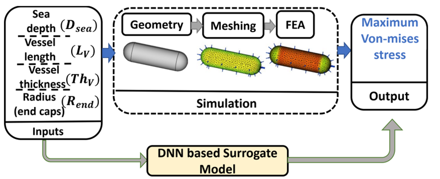
Figure 2. a subsea pressure vessel design based on machine learning [4]
In addition, Ilker used Artificial Neural Network (ANN) to predict the surge pressure in piping systems. The underlying impulse of this study was to create accurate estimation in the initial stage of a project namely Pre-FEED because in this stage there was no sufficient data to either foresee surge pressure or conduct transient analysis, thereby, data of surge pressure obtained from previous projects was used. Thus, the author merely used simple parameters to predict the surge pressure, including pipe segment length, pipe diameter, and pipe location or elevation[5].
A trend of surrogate models based on machine learning and FEA keeps increasing due to the superb ability of the surrogate models in assessing equipment performance swiftly. Di et al [6], designed a surrogate model to predict the maximum stress of the off-center casing which invariably applied in non-uniform ground, the devised machine learning model aimed to replace the expensive experimental methods. 120 samples were yielded from FEM using ANSYS software, then these samples were trained with the Support Vector Machine algorithm, and the results delineated that the proposed model of SVM was capable to predict the von mises stress with relative errors by 0.33% and 0.98%.
Equipment Monitoring
Shandu et al [7]conducted an experiment in monitoring speed of a pump using sensors attached on it. The objective was to provide early warnings to the pump-piping system since invariably pump would operate at excess speed which yielded vibration and led to the emergence of crack due to the cyclic loads (continuous loads at a lower stress than a yield stress of a material). 12 sensors were attached on locations which were vulnerable to the emergence of crack such as elbows, nozzles, and pipe sections where these. The changes of dynamic characteristics in the pump-piping system were recorded and represented in acceleration-time series as a common approach in structural health monitoring as can be seen in figure 3. Artificial Neural Network was used to predict the exact degrade locations in the piping system. Subsequently, further assessments were conducted based on Finite Element Analysis to generate bending stresses of the degrade locations in the pump-piping system which had been predicted by Deep Learning. 2 recommendations were given after conducting the finite element analysis, including the maximum speed of a pump to be operated was 882 rpm, and the maximum hours of a pump to be operated in a day could not surpass 5.6 hours.

Figure 3. Pump-piping monitoring systems [7]
Thomas et al [8]designed a machine learning model to predict the crack depth of specimens which was given thermo-mechanical loads. The interplay between dynamic responses of specimens and crack depth were obtained where the lower the natural frequency the larger the depth of crack which construed the damage location in specimens. In order to acquire dynamic responses of natural frequency then dynamic response measurement tools such as an accelerometer and laser vibrometer were used. According to results the generalised linear model was capable to foresee the crack depth of specimens and the most imperative feature was natural frequency which influenced the model considerably.
Poojitha [9]proposed a machine learning model to predict the dynamic responses of a beam. The objective of this study was to create a surrogate model which could supersede FEA simulation in the future, thereby, this model enabled to conduct real-time monitoring systems. The author obtained initial data of accelerations in the beam by using accelerometers, subsequently this data was processed in FEA to obtain further information regarding accelerations in more wide locations of the beam when loads applied. Random forest and ANN were 2 proposed models which could accurately foresee the dynamic responses in the beam.
Zajam et al [10]proposed a machine learning model namely Support Vector Machine (SVM) classifier to predict the damage location in pipelines. In general, Pipeline Inspection Gauge (PIG) could be used by inserting it in pipelines acted as a load, subsequently, a seismic sensor namely accelerometer was mounted on pipelines. However, in order to diminish the costs required in conducting research and enhance the analysis time, then Finite element analysis with ANSYS software was conducted to generate time-acceleration data with 95 different cases of damage. Then, this data would be processed into Wavelet function which furnished the time and frequency information from 1 to 0. The abrupt changes in wavelet analysis construed there was damage in pipelines. In addition, this information was trained in SVM, whereby damage pipe locations were classified as 1 and vice versa.
The incorporation of machine learning and simulation based software is immensely helpful in establishing swift decisions in fields since the 2 major hindrances of simulation based software such as ABAQUS or ANSYS are time consuming and using this software requires proprer domain expertise which hinders its extensive application. For example, Yang et al[11] developed a web-based dash visualization tool as ehxibited in figure 2. Whereby, this tool is useful in assisting engineers or operators to assess maximum corrosion rates in a pipe bend. The underlying algorithms of this website stems from the machine learning classification algorithm namely LightGBM and MLPNN, where data samples were obtained from CFD simulation

Figure 4. Web based assessment tool [11]
Conclusions
In conclusions, the emergence of machine learning provides solutions to solve issues either in the finite element method or conventional assessment method. The incorporation of machine learning with current methods/tools in assessing mechanical equipment in plants probably enhances the safety and deters failures of equipment. Therefore, incessant development in this field is arguably imperative both in research and application stages since it seems there are many untapped potential to apply this technology in this field.
References
[1] American Society of Mechanical Engineers, BPVC Section VIII Division 2. 2023.
[2] S. D. V. Kumar, M. L. Y. Kai, T. Arumugam, and S. Karuppanan, “A review of finite element analysis and artificial neural networks as failure pressure prediction tools for corroded pipelines,” Materials, vol. 14, no. 20. MDPI, Oct. 01, 2021. doi: 10.3390/ma14206135.
[3] I. Chakraborty, “Estimating collapse pressure of centralizer subs from machine learning models,” in American Society of Mechanical Engineers, Pressure Vessels and Piping Division (Publication) PVP, American Society of Mechanical Engineers (ASME), 2019. doi: 10.1115/PVP2019-93638.
[4] H. Vardhan and J. Sztipanovits, “Deep Learning-based Finite Element Analysis (FEA) surrogate for sub-sea pressure vessel,” Jun. 2022, [Online]. Available: http://arxiv.org/abs/2206.03322
[5] I. Telci, “Machine learning for early stage piping design.”
[6] Q. F. Di et al., “Artificial intelligence method for predicting the maximum stress of an off-center casing under non-uniform ground stress with support vector machine,” Sci China Technol Sci, vol. 63, no. 12, pp. 2553–2561, Dec. 2020, doi: 10.1007/s11431-019-1694-4.
[7] H. K. Sandhu, S. Srikanth Bodda, S. Sauers, and A. Gupta, “CONDITION MONITORING OF NUCLEAR EQUIPMENT-PIPING USING DEEP LEARNING.”
[8] T. Fleet, K. Kamei, F. He, M. A. Khan, K. A. Khan, and A. Starr, “A machine learning approach to model interdependencies between dynamic response and crack propagation,” Sensors (Switzerland), vol. 20, no. 23. MDPI AG, pp. 1–13, Dec. 01, 2020. doi: 10.3390/s20236847.
[9] P. V. Badarinath, M. Chierichetti, and F. D. Kakhki, “A machine learning approach as a surrogate for a finite element analysis: Status of research and application to one dimensional systems,” Sensors, vol. 21, no. 5, pp. 1–18, Mar. 2021, doi: 10.3390/s21051654.
[10] S. Zajam, T. Joshi, and B. Bhattacharya, “Application of wavelet analysis and machine learning on vibration data from gas pipelines for structural health monitoring,” in Procedia Structural Integrity, Elsevier B.V., 2019, pp. 712–719. doi: 10.1016/j.prostr.2019.05.089.
[11] H. Yang, L. Lu, and K. Tsai, “SPE-201275-MS Machine Learning Based Predictive Models for CO2 Corrosion in Pipelines With Various Bending Angles,” 2020.
-
Pressure Vessel Design and Optimization
PRESSURE VESSEL DESIGN
Pressure vessel design commonly refers to ASME Section VII division 1 [1] as international standardization procedures to devise and manufacture a pressure vessel. ASME Boiler and Pressure Vessel Code (BPVC) was issued in 1914 and published in 1915 at the first time, and this standardization covers industrial and residential boilers as well as nuclear reactor components, transportation tanks, and pressure vessels. In pressure vessel design, this standardization is utilized to devise pressurize parts, on the other hand in order to design non-pressurize parts such as a saddle, one can refer to a guidance book of pressure vessel design by Dennis R. Moss[2]. In essence, the determination of pressure vessel thickness is a foremost stage during the design processes, several thickness parts which need to be prescribed, including a shell, head, and nozzle.
Figure 1 exhibits a horizontal pressure vessel as separator with capacity of 3 MMSCFD. This pressure vessel was designed to withstand against internal design pressure of 4.1 MPa, and Internal design temperature of 93oC. SA 516 Gr.70 was selected as the material of a shell and heads. In addition, SA 106 Gr.B was selected to be nozzle materials for Nozzle 1 and Nozzle 2. ASME Sec VII Div 1 underlay the design equations in determining the thickness, MAWP and MAP. Maximum Allowable Working Pressure is the maximum allowed pressure at a specific temperature where a pressure vessel is allowed to be operated. Moreover, Maximum Allowable Pressure (MAP) is the maximum of a pressure vessel in the new and cold condition.
Figure 2 shows the results and comparison between the manual calculation and PV elite analysis. In which, PV elite is common software used in industrial application to assess the design of pressure vessel [3]. From these results, all parts of the pressure vessel complied the standardization codes since the MAWP and MAP were larger than the design pressure [1]. This comparison of results between manual calculation and PV elite analysis is indispensable to be assessed, notably to muster information regarding the percentage variation and observe the permissible range of the output values [4] .

Figure 1. Pressure Vessel (Separator) with capacity of 3MMSCFD

Figure 2. The comparison results between manual calculation and PV Elite.
PRESSURE VESSEL DESIGN OPTIMIZATIONS.
1.) Composite Materials in Pressure Vessels.
Material selections in designing a pressure vessel can be immensely challenging since the proper materials might reduce the weight of pressure vessels and increase the strength of materials. Composite materials are widely utilized to be surrogate materials for pressure vessel application, these materials are compelling due to their superb directional strength, stiffness-to-density ratios, and exceptional physical properties[5] . Composite materials are categorized as anisotropic in which the properties of materials rely to the direction of the load (direction-dependent), conversely common conventional metallic materials are isotropic whereby the material properties are alike in all directions. In order to surmount this issue, the anisotropy materials are invariably stacked by layers. A study from Haris et al [6] scrutinized the composite materials, including S-glass/epoxy, Kevlar/epoxy and carbon/epoxy using Finite Element Analysis, as the results the Kevlar/Epoxy was the proper material which could furnish higher laminate efficiency and the fiber utilization factor which can be seen in Figure 3.

Figure 3. Kevlar/Epoxy as the composite material for pressure vessel application
2.) Designed Thickness Optimizations.Thickness optimizations could be one of the hindrances while devising a pressure vessel, occasionally one must ensure that the designed thickness could withstand against internal pressure which invariably can be optimized by increasing its thickness value, however increasing its thickness diminishes its fracture toughness leading to the emergence of rapid crack propagation in the materials. Shahani et al [7] analyzed the effect of the thickness of steel alloy to its fracture toughness, which is depicted in figure 4. There were optimal values between the fracture toughness and thickness of the material, when the thickness was increased from 1.25 mm to 1.64 mm the plastic zone size to the specimen thickness increased, this result can be construed that the more energy could be absorbed, hence the material could reduce the likelihood of crack propagation. However, when the material thickness inclined to 4.06 mm the fracture toughness declined as well, thus, this would lead to the escalation of stresses in the crack tip field during the crack propagation.

Figure 4. The relationships between thickness and fracture toughness [7].
In essence, when the pressure vessel thickness is enhanced, subsequently a pressure vessel is probably safe to overcome internal pressure but at the same time it is over-designed. Naweed et al [[8] ] attempted to optimize the Reactor Pressure Vessel (RPV), notably on the closure head part (hemispherical) using a design of experiment method (DOE) with ANSYS software, this research concentrated to study the interplay between the under-designed (considered a Tresca yield criterion) and over-designed situation (considered fracture toughness) under ASME standardizations. The results showed that the thickness of the closure head was altered from 160 mm to 167 mm as can be seen in Figure 3, this value was obtained from the state variables and design variables which consisted of maximum stress intensity and mass of the closure head. The results allow engineers to prevent high thickness values for the materials leading to the high operational costs.

Figure 5. The design optimization off the pressure vessel closure head[8]
REFERENCES
[1] American Society of Mechanical Engineers, “Boiler and Pressure Vessel Code – ASME Section VIII Division 1 ,” 2019.
[2] Dennis R. Moss and Michael Basic, “Pressure Vessel Design Manual,” no. 4th, 2012, doi: https://doi.org/10.1016/C2010-0-67103-3.
[3] C. P. Mahandari and M. Sandi, “MECHANICAL DESIGN OF PRESSURE VESSEL FOR THREE PHASE SEPARATOR USING PV ELITE SOFTWARE.”
[4] M. Vivekanandan, R. Venkatesh, T. Sathish, S. Dinesh, M. Ravichandran, and V. Vijayan, “Pressure Vessel Design using PV-ELITE Software with Manual Calculations and Validation by FEM,” 2019.
[5] Krikanov, “ Composite pressure vessels with higher stiffness.,” vol. 48, pp. 119–127, 2000.
[6] H. H. Mian, G. Wang, U. A. Dar, and W. Zhang, “Optimization of composite material system and lay-up to achieve minimum weight pressure vessel,” Applied Composite Materials, vol. 20, no. 5, pp. 873–889, Oct. 2013, doi: 10.1007/s10443-012-9305-4.
[7] A. R. Shahani, M. Rastegar, M. Botshekanan Dehkordi, and H. Moayeri Kashani, “Experimental and numerical investigation of thickness effect on ductile fracture toughness of steel alloy sheets,” Eng Fract Mech, vol. 77, no. 4, pp. 646–659, Mar. 2010, doi: 10.1016/j.engfracmech.2009.12.017.
[8] M. Naweed, U. T. Murtaza, and W. Siddique, “Design optimization of a closure head for a PWR reactor pressure vessel,” Nuclear Engineering and Design, vol. 383, Nov. 2021, doi: 10.1016/j.nucengdes.2021.111436.
Muhamad Alim
Learning and Sharing

